State of the System: A real number x.
Rule of Evolution: ![]() , where a and b are parameters
which we can fixed at our will but which stay constant during the evolution.
, where a and b are parameters
which we can fixed at our will but which stay constant during the evolution.
Motivations:
Given a well-behaved function g, a point y
and a sufficiently small value of x,
we have ![]() where a and b
can be calculated with the help of
calculus (it is called a Taylor expansion). In other words, at
a sufficiently small scale, a curve looks like straight line.
where a and b
can be calculated with the help of
calculus (it is called a Taylor expansion). In other words, at
a sufficiently small scale, a curve looks like straight line.
``Real Life'' Example:
A simple application of the linear map is the following. Let us
call ![]() the amount of money deposited in a bank at a given time,
the amount of money deposited in a bank at a given time,
![]() the amount of money on the account a year after,
the amount of money on the account a year after,
![]() the amount of money on the account two years after, etc...
To calculate
the amount of money on the account two years after, etc...
To calculate ![]() ,
, ![]() , we assume that an interest of 5 percent
is added every year, that the bank gives a fixed amount (say 1 dollar)
every year to its customers and that no additional money is deposited.
The evolution rule is then
, we assume that an interest of 5 percent
is added every year, that the bank gives a fixed amount (say 1 dollar)
every year to its customers and that no additional money is deposited.
The evolution rule is then ![]() .
.
Main Result:
If ![]() , the system has a fixed point
, the system has a fixed point ![]() such that
if
such that
if ![]() , then
, then ![]() .
We can discuss the evolution using either graphical methods (see
``graphical representation .. `` below) or by algebraic methods.
If we write
.
We can discuss the evolution using either graphical methods (see
``graphical representation .. `` below) or by algebraic methods.
If we write ![]() ,
, ![]() , etc. , then
a little algebra shows that
, etc. , then
a little algebra shows that
![]() . It is easy to study the series
. It is easy to study the series ![]() .
If b<0, the signs altenate otherwise the series is the same as for |b|.
If |b|<1 then
.
If b<0, the signs altenate otherwise the series is the same as for |b|.
If |b|<1 then ![]() becomes smaller and smaller when n increases and
becomes smaller and smaller when n increases and
![]() tends to its fixed point value. Such a fixed point is called
attractive.
if |b|>1 then
tends to its fixed point value. Such a fixed point is called
attractive.
if |b|>1 then ![]() becomes larger and larger, and
becomes larger and larger, and ![]() moves
away from the fixed point. Such a fixed point is
called repulsive.
When the fixed point is repulsive, if you start on the right of
the fixed point you move farther right when n increases.
But if you start on the left of
the fixed point, you move farther left.
If b=1, then
moves
away from the fixed point. Such a fixed point is
called repulsive.
When the fixed point is repulsive, if you start on the right of
the fixed point you move farther right when n increases.
But if you start on the left of
the fixed point, you move farther left.
If b=1, then ![]() and
and ![]() goes to
infinity but at a slower rate than when |b|>1
(linear rather than exponential).
If b=-1,
goes to
infinity but at a slower rate than when |b|>1
(linear rather than exponential).
If b=-1, ![]() ,
, ![]() and we are back at our
starting point after two steps. We call this particular type of periodic
behavior a 2-cycle.
and we are back at our
starting point after two steps. We call this particular type of periodic
behavior a 2-cycle.
Important Concepts: Attractive and repulsive fixed point, 2-cycle.
Graphical Representations and Examples
It is often convenient to represent graphically the series ![]() .
For this purpose we draw the function used for the map (here a+bx).
The graph of the function a+bx is a straight line, so we only need
two points to draw it. For instance at x=0, the value of the function
is a and for x=1, the value of the function is a+b.
We then
pick
.
For this purpose we draw the function used for the map (here a+bx).
The graph of the function a+bx is a straight line, so we only need
two points to draw it. For instance at x=0, the value of the function
is a and for x=1, the value of the function is a+b.
We then
pick ![]() on the x-axis, go vertically
to the function, in other words,
we will be at the point
on the x-axis, go vertically
to the function, in other words,
we will be at the point ![]() . We would like to repeat the procedure
with
. We would like to repeat the procedure
with ![]() . In order to do that, we need to move
. In order to do that, we need to move ![]() on the x-axis
and so we move horizontally to the x=y line and we arrive
at the
on the x-axis
and so we move horizontally to the x=y line and we arrive
at the ![]() point. We have now
point. We have now ![]() on the x-axis, we move vertically
to the function and arrive at the point
on the x-axis, we move vertically
to the function and arrive at the point ![]() and so on.
This procedure is illustrated in examples which illustrate the
six cases dicussed above.
and so on.
This procedure is illustrated in examples which illustrate the
six cases dicussed above.
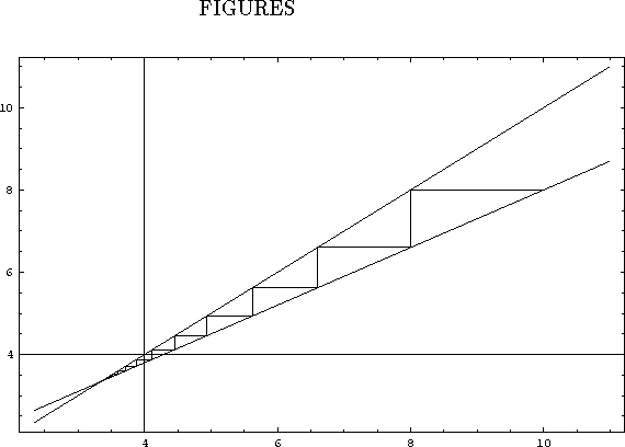
Figure: 10 Iterations of the linear map with a=1, b=0.7 and ![]()
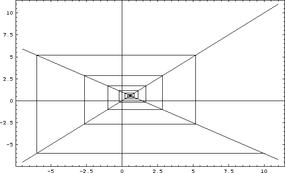
Figure: 10 Iterations of the linear map with a=1, b=-0.7 and ![]()
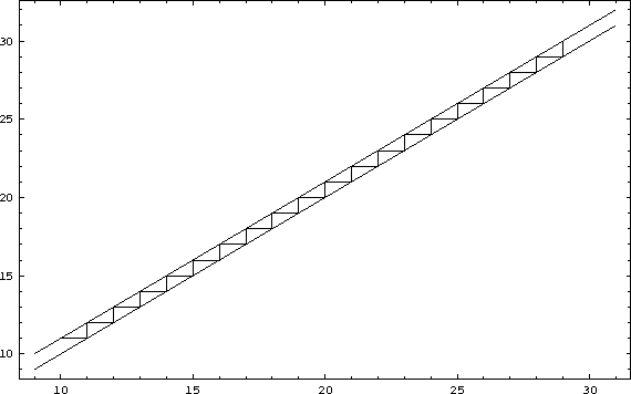
Figure: 10 Iterations of the linear map with a=1, b=1 and ![]()
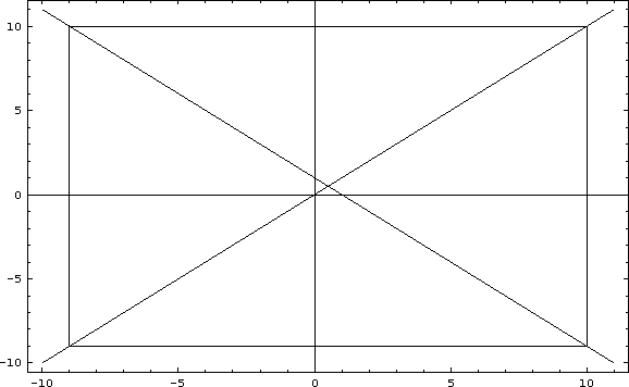
Figure: 10 Iterations of the linear map with a=1, b=-1 and ![]()
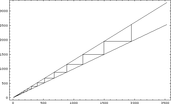
Figure: 10 Iterations of the linear map with a=1, b=1.3 and ![]()
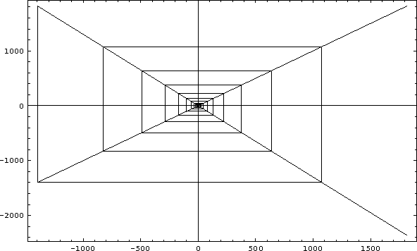
Figure: 10 Iterations of the linear map with a=1, b=-1.3 and ![]()